Sat R-day!: Spatial Statistics and Geostatistics with R
Exploratory data analysis and variography
The Meuse river data contains locations and top soil heavy metal concentrations (ppm), along with a number of soil and landscape variables, collected in a flood plain of the river Meuse, near the village Stein (NLD). The samples are collected from an area of approximately 4.9 km^2^.
In this tutorial, the Zn attribute from the Meuse data set has been examined. This tutorial includes a thematic map of this attribute , histogram of Zn and log(Zn), descriptive statistics, and details about the variogram cloud.
Thematic map
# Required packages
library(sp)           # The meuse data
library(mapview)      # Interactive mapping
library(RColorBrewer) # Custom legend color map package

# Loading and coordinate conversion of the Meuse data
data(meuse)
coordinates(meuse) = ~x+y
proj4string(meuse) <- CRS("+init=epsg:28992")

# This is the mapview function. Note that the legend
# is set to the brewer color palette "Spectral".
meusemap<-mapview(meuse, zcol = "zinc", legend = TRUE,
               cex=4,
               layer.name = 'Zn (ppm)',alpha.regions=0.9,
               col.regions=rev(brewer.pal(11, "Spectral")))
Histogram
library(ggplot2)
library(gridExtra)
library(lattice)

data(meuse)

# Create histogram plot, red dash geom_vline indicates the mean value
hist1<-ggplot(data=meuse, aes(x= meuse$zinc)) +
  geom_histogram(aes(y = after_stat(count / sum(count))*100),bins=15,
                 fill = "skyblue", color = "black")+
    labs(x = "Zn (ppm)", y = "Relative Frequency (%)")+
    theme(panel.border = element_rect(color = "black", fill = NA, size = 1))+
          geom_vline(xintercept = mean(meuse$zinc), size = 1, colour = "#FF3721",
                   linetype = "dashed")

# Get the maximum y axis value
count_values <- ggplot_build(hist1)$data[[1]]$count
max_y<-max(count_values/sum(count_values)*100)

# Histogram of log(Zn (ppm)), y axis limit is set to the max_y
hist2<-ggplot(data=meuse, aes(x= log(meuse$zinc))) +
  geom_histogram(aes(y = after_stat(count / sum(count))*100),bins=15,
                 fill = "blue", color = "black")+
  labs(x = "log(Zn (ppm))", y = "")+
  ylim(0, max_y)+
    theme(panel.border = element_rect(color = "black", fill = NA, size = 1),
          axis.text.y = element_blank())

# Plots are in two columns
grid.arrange(hist1, hist2, ncol = 2)
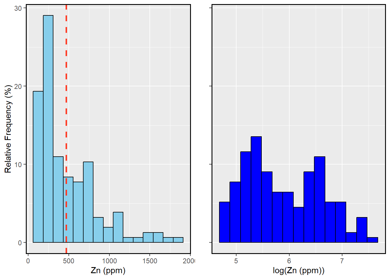
Figure 1: Figure: Histogram of Zn(ppm) and log(Zn(ppm))
Summary statistics
In this section, summary statistics are given in table with a few code lines below.
library(sp)         # Meuse data
library(kableExtra) # Fancy html tables, more info at the references
data(meuse)
# Adding log(Zn) in data frame
d<- data.frame(meuse$zinc, log(meuse$zinc))
names(d)<- c("Zn","log_Zn")

# Summary statistics, then converted into data frame
ds<- summary(d)
dt<- as.data.frame(sapply(d, summary))

# Fixing decimal places 4 and 3 for Zn and log(Zn), respectively
dt$Zn<- signif(dt$Zn, digits = 4)
dt$log_Zn<- signif(dt$log_Zn, digits = 3)

# Renaming row names
row.names(dt) <- c("Minimum","Q1", "Q2 (median)","Mean","Q3","Maximum")

# Arranging the table
kbl(dt) %>%
    kable_styling(bootstrap_options = "striped", full_width = F, position = "left")
| Zn | log_Zn | |
|---|---|---|
| Minimum | 113.0 | 4.73 |
| Q1 | 198.0 | 5.29 |
| Q2 (median) | 326.0 | 5.79 |
| Mean | 469.7 | 5.89 |
| Q3 | 674.5 | 6.51 |
| Maximum | 1839.0 | 7.52 |
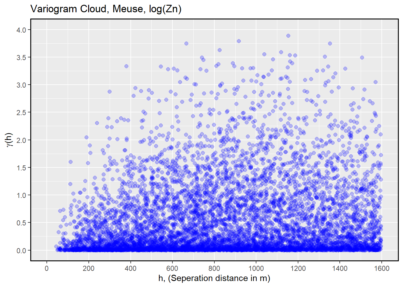
Variography
In geostatistics, a variogram cloud is a graphical representation used to visualize the spatial variability of a variable across a study area.
The following code demonstrates how to visualize a variogram cloud in R using the sp package:
library(sp)
data(meuse)
coordinates(meuse) = ~x+y
plot(variogram(log(zinc)~1, meuse, cloud=TRUE))
In the variogram() function, the default maximum distance is set to one-third of the longest diagonal distance of the data’s bounding box. In the Meuse data set, the bounding box diagonal distance is 4.8 km. Therefore, the default maximum distance is set to 1600 meters.
library(gstat)   # geostatistics package
library(ggplot2) # nice plots

data(meuse)
coordinates(meuse) = ~x+y

# variogram calculation, cloud=TRUE is for cloud scatter
meuse.varioc <- variogram(log(zinc)~1, meuse, cloud=TRUE)


# Customizing the cloud plot
ggplot(meuse.varioc, aes(x=meuse.varioc$dist, y=meuse.varioc$gamma)) +
  geom_point(color = "blue", fill = "blue", size = 2, alpha = 0.25) +
  labs(title = "Variogram Cloud, Meuse, log(Zn)",
       x = "h, (Seperation distance in m)",
       y = expression(paste(gamma, "(h)")))+
  scale_x_continuous(limits = c(0, 1600), breaks = seq(0, 1600, by = 200))+
  scale_y_continuous(limits = c(0, 4), breaks = seq(0, 4, by = 0.5))+
  theme(panel.border = element_rect(color = "black", fill = NA, size = 1))
BONUS: Matlab code for variogram cloud.
clc
clear
close all
% Load the data set and map coordinates
% and the attribute at interest
load meuse
x=data(:,1);
y=data(:,2);
log_zn=data(:,3);

% Bounding box, bb. This is to determine
% the maximum distance.
bb=[min(x) min(y);max(x) max(y)];

% Distance matrix of bounding box.
% Maximum of unique values are extracted
% and maximum value is the diagonal of
% the bounding box.
% Note that default cutoff in gstat
% is one-third of maximum distance
cutoff=max(unique(pdist2(bb,bb)/3));

% Distance matrix between data points
D1=triu(pdist2(data(:,1:2),data(:,1:2)));

% Constraining less than cutoff distances.
% assigning diagonal elements to zero.
% Finally, setting the indexing which pairs
% are satisfying the distance constraint.
D=triu(D1<cutoff);
D(logical(eye(size(D)))) = 0;
index=D(:);

% This is experimental variogram.
% Basically, squared differences
ev = triu(bsxfun(@minus, log_zn, log_zn').^2/2);

% Indexing which pairs are satisfying
% the condition.
var_cloud=[D1(index) ev(index)];

% Plot and plot aesthetics
s=scatter(var_cloud(:,1),var_cloud(:,2),'filled','b');
box on
ylabel('Semi-variogram, \gamma (h)');
xlabel('Seperation distance (m), h');
title('Variogram cloud')
s.MarkerFaceAlpha = 0.25;
ax = gca;
ax.XMinorGrid = 'on';
ax.GridLineStyle='--';
The output image of Matlab code:

Next week, the variography will be discussed more in detail.
Good luck!
References:
- Appelhans, Tim, Florian Detsch, Christoph Reudenbach, and Stefan Woellauer. 2018. Mapview: Interactive Viewing of Spatial Data in R. https://CRAN.R-project.org/package=mapview.
- Pebesma, Edzer, and Roger Bivand. 2018. Sp: Classes and Methods for Spatial Data. https://CRAN.R-project.org/package=sp.
- kableExtra: https://cran.r-project.org/web/packages/kableExtra/vignettes/awesome_table_in_html.html#Overview